Sandpiles
A sandpile is a cellular automaton and dynamical system that displays self-organized criticality. It was introduced by Bak, Tang and Wiesenfeld in 1987.
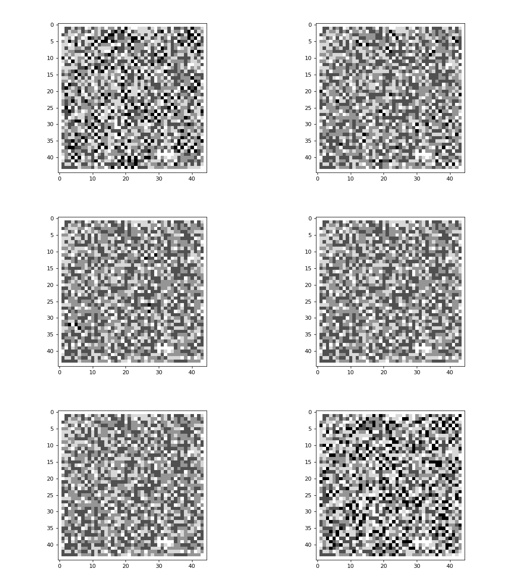
Below is an example of a sandpile using the built-in Sandpile class. The boundary of
the 2D CA can be either closed or open. If the boundary is closed, then all boundary cells should have a value of 0.
import cellpylib as cpl
import numpy as np

n_rows = 45
n_cols = 45
sandpile = cpl.Sandpile(n_rows, n_cols)

ca = np.random.randint(5, size=n_rows*n_cols).reshape((1, n_rows, n_cols))
# we're using a closed boundary, so make the boundary cells 0
ca[0, 0, :], ca[0, n_rows-1, :], ca[0, :, 0], ca[0, :, n_cols-1] = 0, 0, 0, 0

ca = cpl.evolve2d(ca, timesteps=50, apply_rule=sandpile, neighbourhood="von Neumann")

cpl.plot2d_animate(ca)

Note that in the example above, the number of timesteps is fixed at 50. However, for any random initial conditions, it
isn’t obvious how many timesteps are necessary for the system to reach a stable state, or fixed point, in its evolution.
The library provides a function, until_fixed_point(), that can be called to provide a
callable for the timesteps argument of the evolve2d() function. By calling this
function, instead of providing a fixed number, the sandpile will evolve until there is no further change in the state of
the system. Below is an example demonstrating this:
import cellpylib as cpl
import numpy as np
np.random.seed(0)

n_rows = 45
n_cols = 45
sandpile = cpl.Sandpile(n_rows, n_cols)

initial = np.random.randint(5, size=n_rows*n_cols).reshape((1, n_rows, n_cols))
# we're using a closed boundary, so make the boundary cells 0
initial[0, 0, :], initial[0, n_rows-1, :], initial[0, :, 0], initial[0, :, n_cols-1] = 0, 0, 0, 0

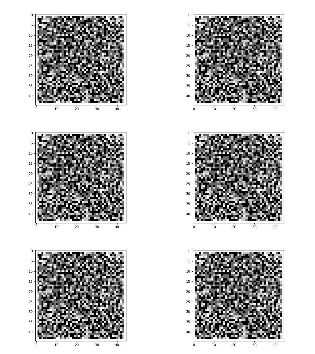
ca = cpl.evolve2d(initial, timesteps=cpl.until_fixed_point(),
                  apply_rule=sandpile, neighbourhood="von Neumann")

print("Number of timesteps to reach fixed point: %s" % len(ca))
cpl.plot2d_animate(ca)
The above program will print out the following:
Number of timesteps to reach fixed point: 51
If one perturbs a sandpile that has reached a fixed point in its evolution, then the sandpile should reconfigure itself
and eventually reach a fixed point once again. This can be demonstrated using the
add_grain() function of the Sandpile class. In the
example below, we begin with a sandpile that has reached a fixed point (this configuration is assumed to exist in a file
called sandpile_add_grain_demo.txt, located in the same directory as the program). We drop a grain of sand on the cell
located at row with index 23 and column with index 23 at timestep 1.
import cellpylib as cpl
import numpy as np

n_rows = 45
n_cols = 45
sandpile = cpl.Sandpile(n_rows, n_cols)
sandpile.add_grain(cell_index=(23, 23), timestep=1)

initial = np.loadtxt('sandpile_add_grain_demo.txt', dtype=int)
initial = np.array([initial])

ca = cpl.evolve2d(initial, timesteps=cpl.until_fixed_point(),
                  apply_rule=sandpile, neighbourhood="von Neumann")

print("Number of timesteps to reach fixed point: %s" % len(ca))
cpl.plot2d_animate(ca)

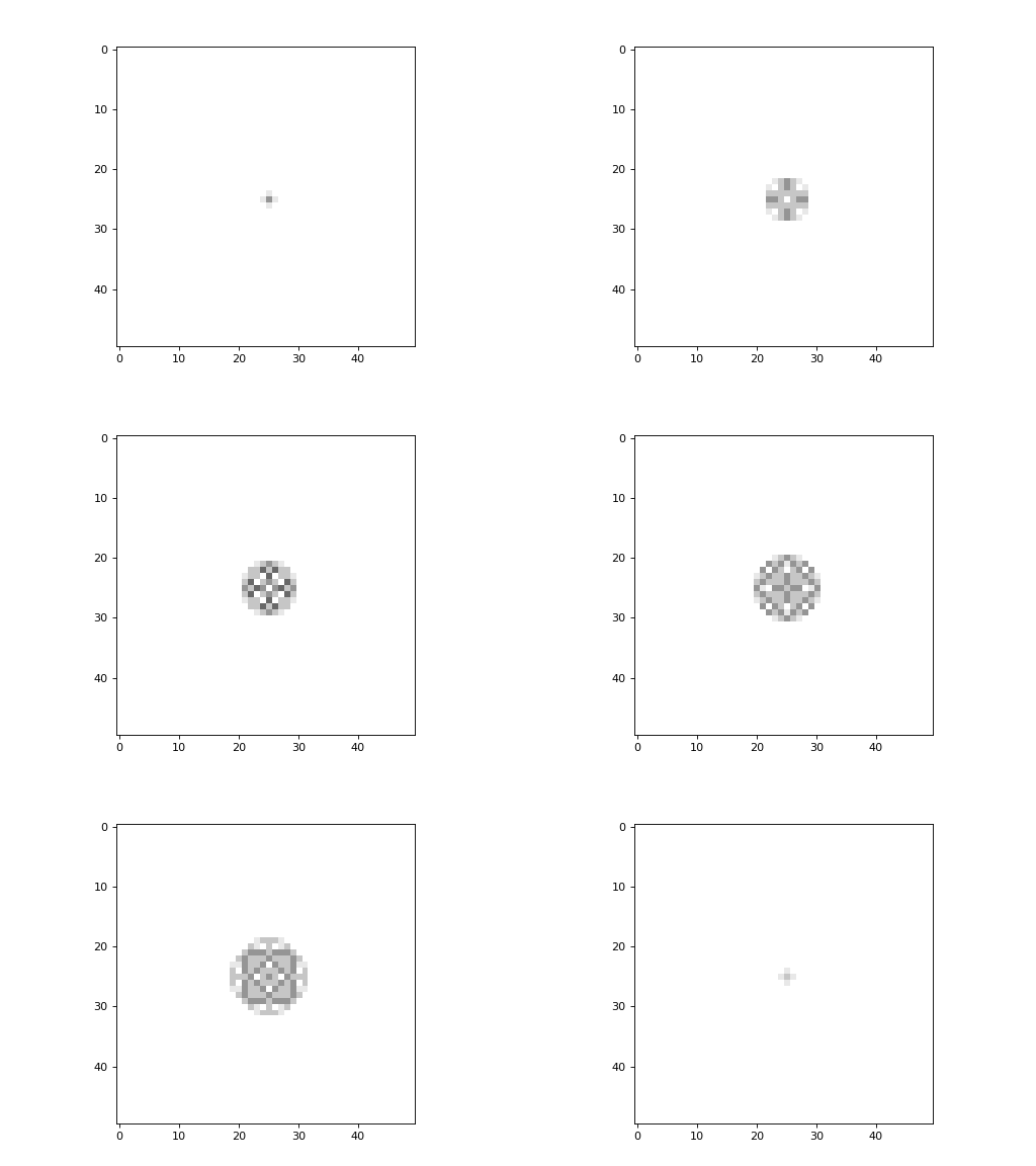
Imagine dropping a single grain of sand repeatedly on the same cell in the center of a grid, allowing the sandpile to attain a stable state (i.e. fixed point) before dropping the next grain. This can be demonstrated with the following code snippet:
import cellpylib as cpl

n = 50
sandpile = cpl.Sandpile(n, n)
ca = cpl.init_simple2d(n, n, val=5)

for i in range(300):
    ca[-1, n//2, n//2] += 1
    ca = cpl.evolve2d(ca, apply_rule=sandpile,
                      timesteps=cpl.until_fixed_point(), neighbourhood='Moore')

cpl.plot2d_animate(ca)

Above, we take advantage of the fact that the ca argument to evolve2d() can
contain a history of prior states, and that the evolution continues from the last state.
References:
Bak, Per, Chao Tang, and Kurt Wiesenfeld. “Self-organized criticality.” Physical review A 38.1 (1988): 364.