Additional Features

Langton’s Lambda

One way to specify CA rules is with rule tables. Rule tables are enumerations of all possible neighbourhood states together with their cell state mappings. For any given neighbourhood state, a rule table provides the associated cell state value. CellPyLib provides a built-in function for creating random rule tables. The following snippet demonstrates its usage:

import cellpylib as cpl

rule_table, actual_lambda, quiescent_state = cpl.random_rule_table(lambda_val=0.45, k=4, r=2,
                                                                   strong_quiescence=True,
                                                                   isotropic=True)
cellular_automaton = cpl.init_random(128, k=4)

# use the built-in table_rule to use the generated rule table
cellular_automaton = cpl.evolve(cellular_automaton, timesteps=200,
                                apply_rule=lambda n, c, t: cpl.table_rule(n, rule_table), r=2)

The following plots demonstrate the effect of varying the lambda parameter:

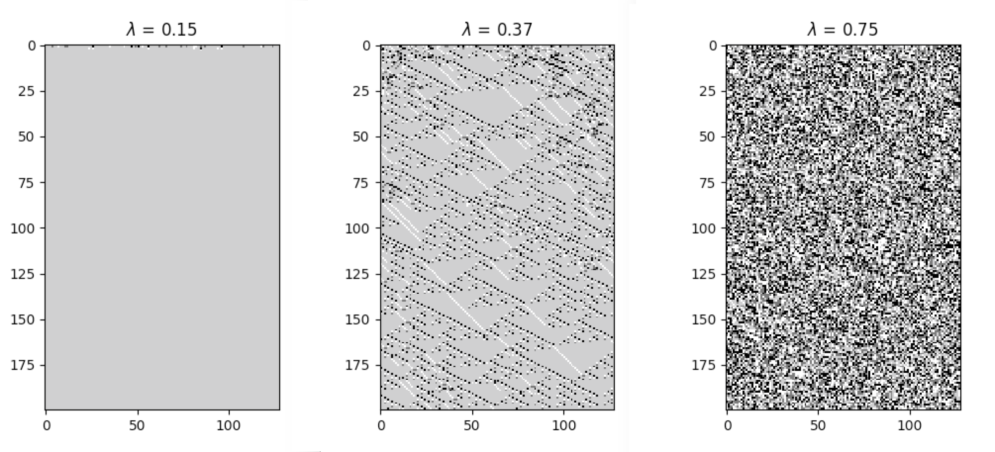
C. G. Langton describes the lambda parameter, and the transition from order to criticality to chaos in cellular automata while varying the lambda parameter, in the paper:

Langton, C. G. (1990). Computation at the edge of chaos: phase transitions
and emergent computation. Physica D: Nonlinear Phenomena, 42(1-3), 12-37.

Reversible CA

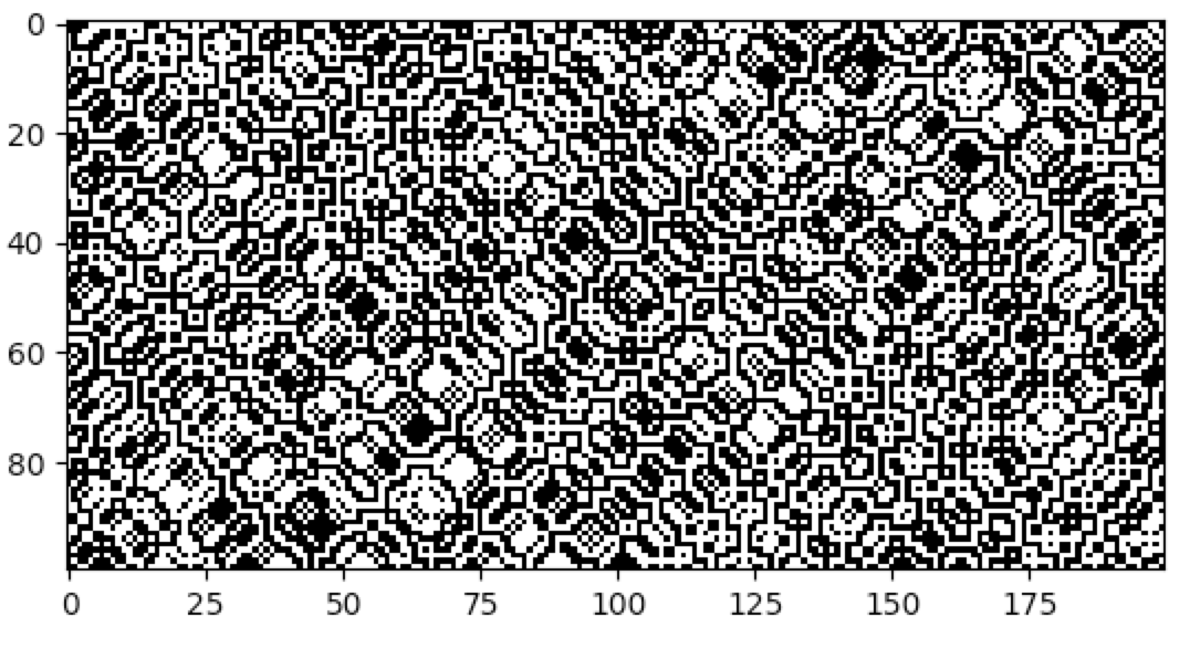
Elementary CA can be explicitly made to be reversible. CellPyLib has a class, ReversibleRule, which can be used to decorate a rule, making it reversible. The following example demonstrates the creation of the elementary reversible CA rule 90R:

import cellpylib as cpl

cellular_automaton = cpl.init_random(200)
rule = cpl.ReversibleRule(cellular_automaton[0], 90)

cellular_automaton = cpl.evolve(cellular_automaton, timesteps=100,
                                apply_rule=ule)

cpl.plot(cellular_automaton)

Asynchronous CA

Typically, evolving a CA involves the synchronous updating of all the cells in a given timestep. However, it is also possible to consider CA in which the cells are updated asynchronously. There are various schemes for achieving this. Wikipedia has a page dedicated to this topic.

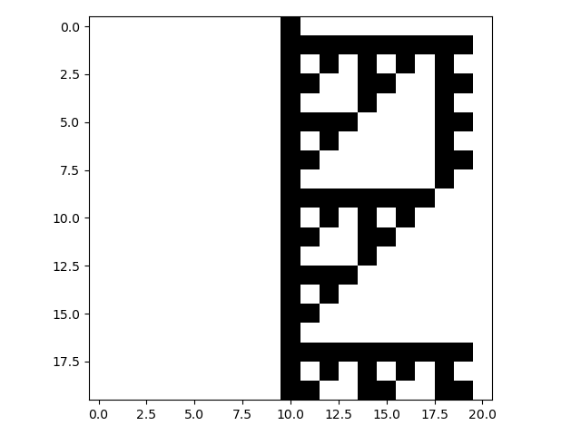
CellPyLib has a class, AsynchronousRule, which can be used to decorate a rule, making it asynchronous. In the following example, the rule 60 sequential CA from the notes of A New Kind of Science (Chapter 9, section 10: Sequential cellular automata) is implemented:

import cellpylib as cpl

cellular_automaton = cpl.init_simple(21)

rule = cpl.AsynchronousRule(apply_rule=lambda n, c, t: cpl.nks_rule(n, 60),
                         update_order=range(1, 20))

cellular_automaton = cpl.evolve(cellular_automaton, timesteps=19*20,
                                apply_rule=rule)

# get every 19th row, including the first, as a cycle is completed every 19 rows
cpl.plot(cellular_automaton[::19])

The AsynchronousRule requires the specification of an update order (if none is provided, then an order is constructed based on the number of cells in the CA). An update order specifies which cell will be updated as the CA evolves. For example, the update order [2, 3, 1] states that cell 2 will be updated in the next timestep, followed by cell 3 in the subsequent timestep, and then cell 1 in the timestep after that. This update order is adhered to for the entire evolution of the CA. Cells that are not being updated do not have the rule applied to them in that timestep.

An option is provided to randomize the update order at the end of each cycle (i.e. timestep). This is equivalent to selecting a cell randomly at each timestep to update, leaving all others unchanged during that timestep. The following example demonstrates a simplistic 2D CA in which a cell is picked randomly at each timestep, and its state is updated to a value of 1 (all cells begin with a state of 0):

import cellpylib as cpl

cellular_automaton = cpl.init_simple2d(50, 50, val=0)

apply_rule = cpl.AsynchronousRule(apply_rule=lambda n, c, t: 1, num_cells=(50, 50),
                                  randomize_each_cycle=True)

cellular_automaton = cpl.evolve2d(cellular_automaton, timesteps=50,
                                  neighbourhood='Moore', apply_rule=apply_rule)

cpl.plot2d_animate(cellular_automaton, interval=200, autoscale=True)

CTRBL Rules

There exists a class of important CA that exhibit the property of self-reproduction. That is, there are patterns observed that reproduce themselves during the evolution of these CA. This phenomenon has obvious relevance to the study of Biological systems. These CA are typically 2-dimensional, with a von Neumann neighbourhood of radius 1. The convention when specifying the rules for these CA is to enumerate the rule table using the states of the center (C), top (T), right (R), bottom (B), and left (L) cells in the von Neumann neighbourhood.

Such CTRBL CA are supported in CellPyLib, through the CTRBLRule class. A particularly well-known CA in this class is Langton’s Loop. CellPyLib has a built-in implementation of this CA, available through the LangtonsLoop class.

Here is a simple example of a 2D CA that uses a CTRBL rule:

import cellpylib as cpl

ctrbl_rule = cpl.CTRBLRule(rule_table={
    (0, 1, 0, 0, 0): 1,
    (1, 1, 0, 0, 0): 0,
    (0, 0, 0, 0, 0): 0,
    (1, 0, 0, 0, 0): 1,
    (0, 0, 1, 1, 0): 0,
    (1, 1, 1, 1, 1): 1,
    (0, 1, 0, 1, 0): 0,
    (1, 1, 1, 0, 1): 1,
    (1, 0, 1, 0, 1): 1,
    (0, 1, 1, 1, 1): 1,
    (0, 0, 1, 1, 1): 0,
    (1, 1, 0, 0, 1): 1
}, add_rotations=True)

cellular_automaton = cpl.init_simple2d(rows=10, cols=10)

cellular_automaton = cpl.evolve2d(cellular_automaton, timesteps=60,
                                  apply_rule=ctrbl_rule, neighbourhood="von Neumann")

cpl.plot2d_animate(cellular_automaton)

It is a binary CA that always appears to evolve to some stable attractor state.

Custom Rules

A rule is a callable that contains the logic that will be applied to each cell of the CA at each timestep. Any kind of callable is valid, but the callable must accept 3 arguments: n, c and t. Furthermore, the callable must return the state of the current cell at the next timestep. The n argument is the neighbourhood, which is a NumPy array of length 2r + 1 representing the state of the neighbourhood of the cell (for 1D CA), where r is the neighbourhood radius. The state of the current cell will always be located at the “center” of the neighbourhood. The c argument is the cell identity, which is a scalar representing the index of the cell in the cellular automaton array. Finally, the t argument is an integer representing the time step in the evolution.

Any kind of callable is supported, and this is particularly useful if more complex handling, like statefulness, is required by the rule. For complex rules, the recommended approach is to define a class for the rule, which provides a __call__ function which accepts the n, c, and t arguments. The BaseRule class is provided for users to extend, which ensures that the custom rule is implemented with the correct __call__ signature.

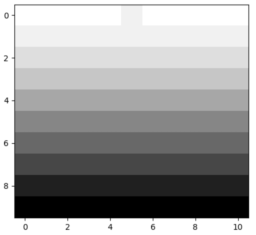
As an example, below is a custom rule that simply keeps track of how many times each cell has been invoked:

import cellpylib as cpl
from collections import defaultdict

class CustomRule(cpl.BaseRule):

    def __init__(self):
        self.count = defaultdict(int)

    def __call__(self, n, c, t):
        self.count[c] += 1
        return self.count[c]

rule = CustomRule()

cellular_automaton = cpl.init_simple(11)

cellular_automaton = cpl.evolve(cellular_automaton, timesteps=10,
                                apply_rule=rule)

cpl.plot(cellular_automaton)