Block CA and The Second Law
In a typical CA, each cell is processed one-by-one, taking into account its surrounding neighbourhood cells. However, in Block CA, the cells are processed in groups known as blocks. The rules of Block CA do not act on a single cell, but rather act on each block of cells as a whole. With this format, it becomes easier to set up rules which are reversible and which conserve quantities, such as cell colors. This makes Block CA useful for emulating physical systems.
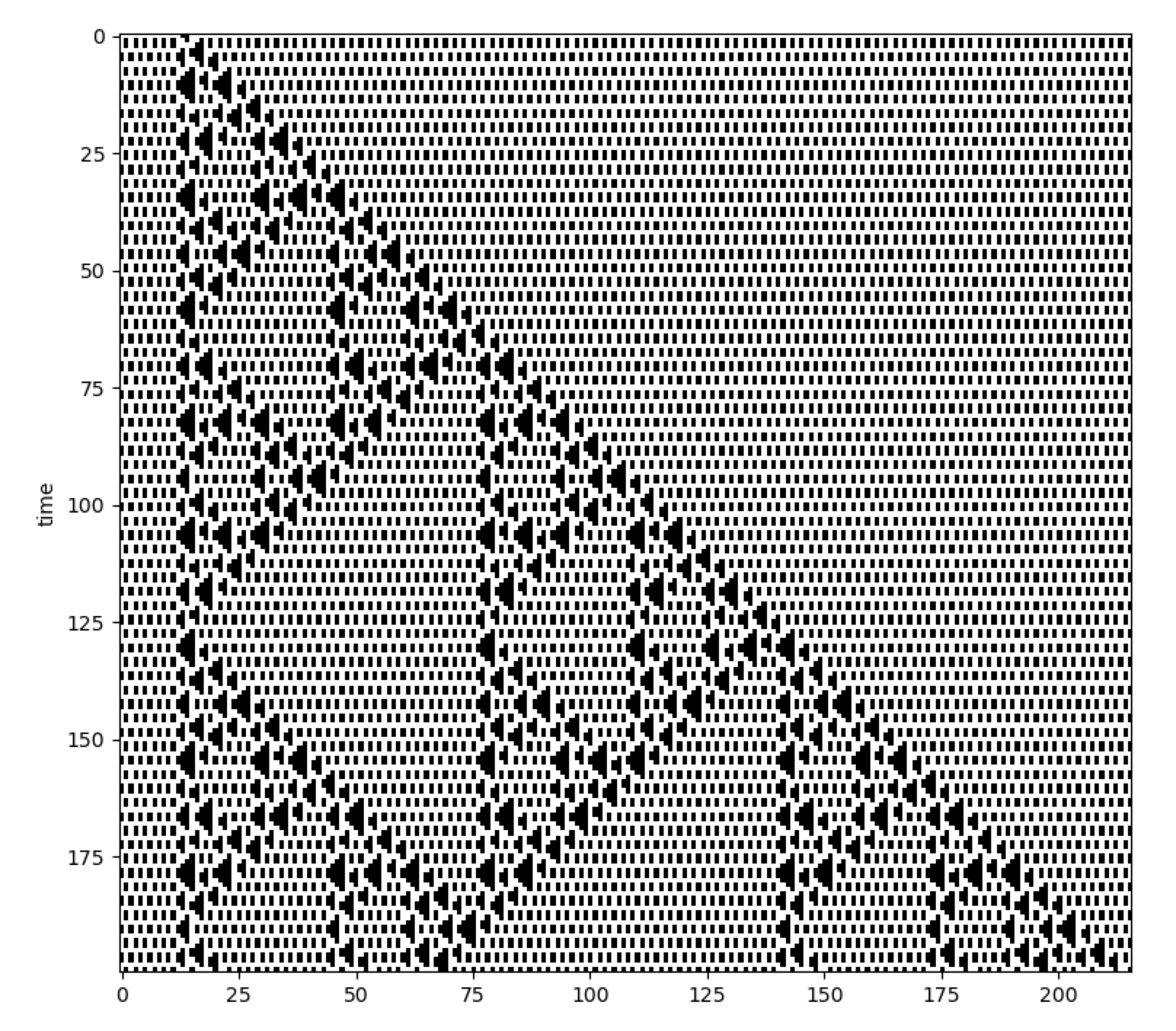
Below is an example of a Block CA implemented with CellPyLib, which makes use of the built-in function
evolve_block(). This CA was taken from Stephen Wolfram’s book A New Kind of Science,
on page 460:
import cellpylib as cpl
import numpy as np

initial_conditions = np.array([[0]*13 + [1]*2 + [0]*201])

def block_rule(n, t):
    if n == (1, 1): return 1, 1
    elif n == (1, 0): return 1, 0
    elif n == (0, 1): return 0, 0
    elif n == (0, 0): return 0, 1

ca = cpl.evolve_block(initial_conditions, block_size=2,
                      timesteps=200, apply_rule=block_rule)

cpl.plot(ca)
Block CA can be comprised of more than two colors, as the following example demonstrates, taken from Stephen Wolfram’s book A New Kind of Science, on the bottom of page 462:
import cellpylib as cpl
import numpy as np

initial_conditions = np.array([[0]*30 + [2]*30 + [0]*30])

def block_rule(n, t):
    if   n == (1, 1): return 1, 1
    elif n == (1, 0): return 0, 2
    elif n == (0, 1): return 2, 0
    elif n == (0, 0): return 0, 0
    elif n == (2, 2): return 2, 2
    elif n == (2, 0): return 1, 0
    elif n == (0, 2): return 0, 1
    elif n == (2, 1): return 2, 1
    elif n == (1, 2): return 1, 2

ca = cpl.evolve_block(initial_conditions, block_size=2,
                      timesteps=4500, apply_rule=block_rule)

cpl.plot(ca[-500:])
The Second Law
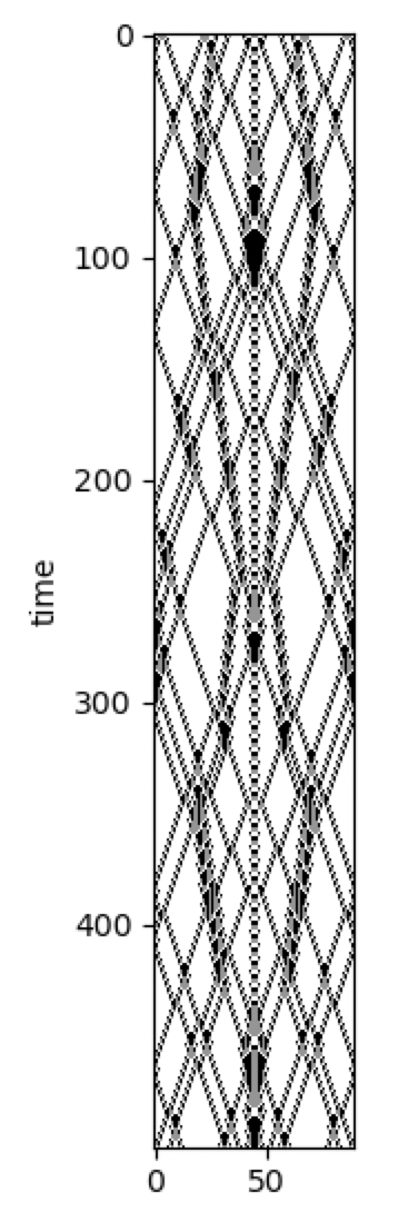
In a series of articles, Stephen Wolfram shared his thoughts on the computational origins of the Second Law of Thermodynamics. In the first part of the series, he illustrates his ideas with a number of different Block CA, such as the one shown here:
The code for this Block CA is given below:
import cellpylib as cpl
import numpy as np

initial_conditions = np.array([[0]*25 + [2]*17 + [0]*24])

def block_rule(n, t):
    if   n == (1, 1): return 2, 2
    elif n == (1, 0): return 1, 0
    elif n == (0, 1): return 0, 1
    elif n == (0, 0): return 0, 0
    elif n == (2, 2): return 1, 1
    elif n == (2, 0): return 0, 2
    elif n == (0, 2): return 2, 0
    elif n == (2, 1): return 2, 1
    elif n == (1, 2): return 1, 2

ca = cpl.evolve_block(initial_conditions, block_size=2,
                      timesteps=200, apply_rule=block_rule)

cpl.plot(ca)
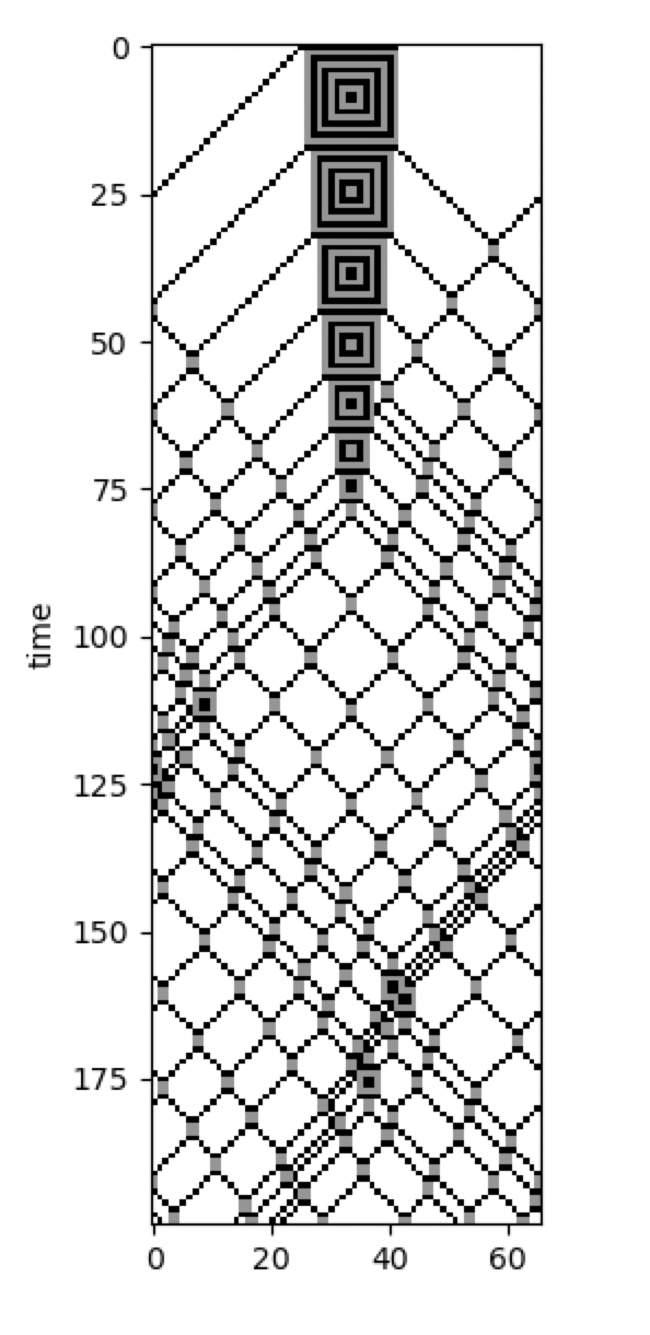
Simple cellular automata systems with reversible and color-conserving rules give rise to the same “randomization” seen in physical systems consisting of diffusing particles, as this “gas-like” 2D Block CA demonstrates:
CellPyLib supports 2D Block CA through the built-in function evolve2d_block().
The code for this 2D Block CA is given below:
import cellpylib as cpl
import numpy as np

# visit https://github.com/lantunes/cellpylib/tree/master/demos
#  for the initial conditions file
initial_conditions = np.loadtxt('block2d_rotated_initial_conditions.txt', dtype=int)
initial_conditions = np.array([initial_conditions])

def make_block2d_rule():
    base_rules = {
        ((0, 0), (0, 0)): ((0, 0), (0, 0)),
        ((0, 0), (0, 2)): ((2, 0), (0, 0)),
        ((2, 0), (0, 0)): ((0, 0), (0, 2)),
        ((0, 0), (2, 0)): ((0, 2), (0, 0)),
        ((0, 2), (0, 0)): ((0, 0), (2, 0)),
        ((0, 0), (2, 2)): ((2, 2), (0, 0)),
        ((2, 2), (0, 0)): ((0, 0), (2, 2)),
        ((0, 2), (0, 2)): ((2, 0), (2, 0)),
        ((2, 0), (2, 0)): ((0, 2), (0, 2)),
        ((0, 2), (2, 0)): ((2, 0), (0, 2)),
        ((2, 0), (0, 2)): ((0, 2), (2, 0)),
        ((0, 2), (2, 2)): ((2, 2), (2, 0)),
        ((2, 2), (2, 0)): ((0, 2), (2, 2)),
        ((2, 0), (2, 2)): ((2, 2), (0, 2)),
        ((2, 2), (0, 2)): ((2, 0), (2, 2)),
        ((2, 2), (2, 2)): ((2, 2), (2, 2)),
        # wall rules
        ((0, 0), (1, 1)): ((0, 0), (1, 1)),
        ((0, 1), (1, 1)): ((0, 1), (1, 1)),
        ((0, 2), (1, 1)): ((2, 0), (1, 1)),
        ((2, 0), (1, 1)): ((0, 2), (1, 1)),
        ((2, 1), (1, 1)): ((2, 1), (1, 1)),
        ((2, 2), (1, 1)): ((2, 2), (1, 1)),
        ((1, 1), (1, 1)): ((1, 1), (1, 1)),
        ((1, 0), (0, 0)): ((1, 0), (0, 0)),
        ((1, 0), (0, 2)): ((1, 0), (0, 2)),
    }
    rules = {}
    # add rotations
    for r, v in base_rules.items():
        rules[r] = v
        for _ in range(3):
            r = ((r[1][0], r[0][0]), (r[1][1], r[0][1]))
            v = ((v[1][0], v[0][0]), (v[1][1], v[0][1]))
            if r not in rules:
                rules[r] = v
    def _apply_rule(n, t):
        n = tuple(tuple(i) for i in n)
        return rules[n]
    return _apply_rule

ca = cpl.evolve2d_block(initial_conditions, block_size=(2, 2),
                        timesteps=251, apply_rule=make_block2d_rule())

cpl.plot2d_animate(ca)
References:
https://en.wikipedia.org/wiki/Block_cellular_automaton
https://www.wolframscience.com/nks/p459–conserved-quantities-and-continuum-phenomena/